Recently, many friends asked me how to understand SVM intuitively. They were confused by the complicated mathematical formulas. Today I will thoroughly explain what is SVM through eight questions. For those who need to know the mathematical proofs, please refer to the appendix below.
Q1: How to understand SVM most intuitively?
Ans1: Firstly, take a look at the chart below. SVM is a classifier(can be regressor as well) to classify data by generating a decision boundary or hyperplane(the red line below) with the biggest margin and separate the data with different classes into the opposite side of the boundary. Actually, we can have two parallel hyperplanes that separate the different data into the opposite side and the distance between them should be as large as possible. The region bounded by these two hyperplanes is called the margin, and the most robust decision boundary is the hyperplane that lies halfway between them. The data lies on the two parallel hyperplanes are called support vector.

Q2: What is the nature of SVM from a math perspective?
Ans2: SVM is a typical convex quadratic programming problem. It tries to find a solution to minimize the margin subject to the constraint that all data with different classes stay on the opposite side of the boundary. The following formula is the objective function of the standard SVM. For math details please reference the Appendix below.

Q3: What are hard-margin and soft-margin?
Ans3: For linearly separable data the standard SVM algorithm has a solution. This standard SVM as we described above is hard-margin SVM. However, when the data is approximately linearly separable but not exact linearly separable, standard SVM fails. We can slightly modify the standard SVM to adapt to the new requirement by adding a punishment item in the objective function and decreasing the margin a little bit in the constraint. The advantage of soft-margin SVM is avoiding overfitting and more robust than standard SVM. The following formula is the objective function of the soft-margin SVM.

Q4: What is hinge loss?
Ans4: As we know from Q3, for soft-margin SVM, we will involve a punishment item in the objective function. This punishment item is just the hinge loss. It punishes the data wrong classified by our model. The hinge function is as follows.

Q5: What is the Kernel trick?
Ans5: The kernel trick or kernel method is an elegant skill for converting data from a low dimension space to a higher dimension space by a specific kernel function, which is more computationally efficient than the direct conversion. The purpose of this conversion is to make the linearly inseparable data to be linearly separable in a higher dimension space. Based on this method, SVM is able to handle more linearly inseparable data. The most common kernel functions include Polynomial kernel, Gaussian kernel, Gaussian radial basis function (RBF), Laplace RBF kernel, etc. The following chart shows a linearly inseparable dataset in 2D space that can be linearly separated when it is converted to the 3D space.

Q6: What is the One-class SVM?
Ans6: Suppose the following task, you need to build a classifier to classify dog pictures from a large volume of pictures and you only have dog pictures labeled as the dog. Many smart guys may come up with a strategy that labeling all the rest pictures as non-dog and conduct this task as a normal binary classification problem. It seems like a very good idea. However, if you take a look at the following chart on the left side you will know this idea is not so perfect. The decision boundary generated by the training data will predict the triangle sample as a dog picture since it is also on the same side as dog samples. However, this sample is obviously far away from the dog samples. Consider that the set of non-dog pictures is infinite, the yellow cross samples are just a tiny part of the population. Therefore, the triangle sample is more likely to be a non-dog sample. The right side decision boundary makes more sense since it only focuses on the dog samples, any samples outside the red circle will be predicted as non-dog samples. This intuitive red circle decision boundary involves a very crucial idea of one-class SVM that the one-class SVM only detects the sample that is close to the dog population, other samples will all be considered as non-dog.

We have two models for one-class SVM. One is OCSVM, second is SVDD. The SVDD is more intuitive, whose objective function is just from the idea of the above right picture. It attempts to find a hypersphere with the shortest radius but contains all the labeled samples. This hypersphere is determined by the center and the radius R. Because it has a punishment item or loss, it also belongs to the soft-margin SVM. The objective function of SVDD is as follows.

Q7: What is S3VM?
The standard SVM only applies to supervised learning. A large amount of data generated in real life is unlabeled, and the standard form of SVM cannot make good use of these data to improve its learning ability. However, a semi-supervised support vector machine (S3VM) is a good solution to this problem. The decision boundary of SVM and S3VM can be clearly distinguished by the following chart.
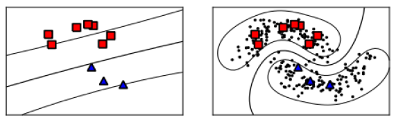
The left picture is the decision boundary of SVM which is a straight line. The right picture is the decision boundary of S3VM which is a curve. The reason for the different decision boundaries is because the S3VM has an extra punishment for those unlabeled data that are close to the decision boundary in the objective function. This extra punishment will make the decision boundary to go through the low-density region since the high-density region contains more unlabeled data. For more details of the objective function please refer to the Appendix.
Q8: What is the cons and pros of SVM?
Pros: 1. SVM is very effective for high dimensional data, even when the number of dimensions is greater than the number of samples. 2. Since the decision boundary is only determined by the support vector which is just a subset of the entire dataset, so it is very memory efficient. Due to the pros SVM is often used in image classification and NLP like sentiment analysis, since those tasks involve large dimensional data.
Cons: 1. SVM is not computationally efficient. It is not suitable for large datasets. 2. SVM is sensitive to noise. It will not perform well if the dataset contains many noisy data. You can consider this con from the perspective of hard-margin and soft-margin. For the hard-margin SVM, a single noisy sample may lead the SVM unsolvable. Therefore, SVM is not suitable for big data projects and noisy data tasks.
